
This blog post is part 2 of a 2 part series exploring the Transformer architecture. Read Part 1 if you haven’t already had the chance.
The Arhitecture (Contd.)
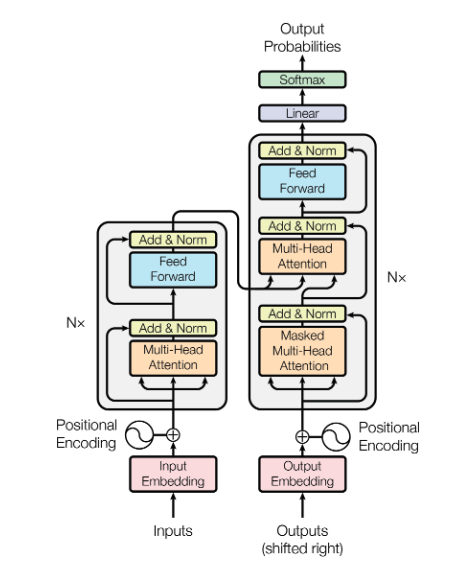
Encoder & Decoders Blocks
In the first part of this explainer, we looked at the Transformer architecture at a high level, learning how the input data gets transformed before entering the main part of the model, the encoder and decoder stacks.
Now, let’s take a deep dive into the components of the encoder and decoder blocks, exploring how they differ from each other and how they are connected. We will focus primarily on the attention mechanism, with some mention of the feed-forward layer, residual connections, and normalization.
Before we dive into the detail of attention, it’s interesting to note that there are two types of attention:
- Self-Attention (with masked and unmasked variants)
- Cross-Attention
Attention Mechanism
So what exactly is attention and what is it doing ?
At an intuitive level, attention helps the model focus on the most important parts of the input sequence. Instead of treating all parts of the input equally, it assigns different weights to different tokens, highlighting which ones are more relevant at each step. This allows the model to dynamically concentrate on crucial bits of information, better capturing relationships and context. Essentially, attention lets the model selectively “pay attention” to the parts of the input that matter most, making its understanding and output more accurate and context-aware.
As we mentioned earlier there’s more than one type of attention layer in the Transformer architecture, all with the same core but with minor differences, we have:
- Self-Attention (un-masked)
- Self-Attention (masked)
- Cross-Attention
Self-Attention
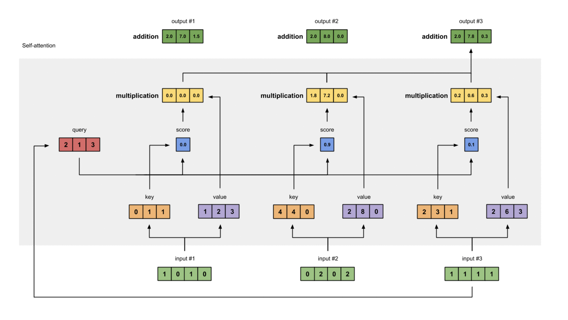
Great! Now that we know what it’s doing, let’s take a look at how it works. What are the steps involved ?
- Prepare our inputs as described in part 1.
- Initialise some weights in 3 projection matrices: $W^Q, W^K, W^V$
- Multiply our inputs against these matrices to get a key ($Q$), query ($K$) and value ($V$) vectors.
- Take the dot product between the key and query vectors to get an attention score. The dot product is essentially calculating some semantic similarity between these vectors.
- Apply the softmax function to the attention score to normalise them into probabilities (i.e everything sums to 1) .
- Multiply our matrix of attention scores (”probabilities”) by the value vectors to get a weighted influence of each surrounding token.
- Finally, sum these weighted value vectors to produce the output vector.
Basically each word (token) is learning about / influencing each other to some extent, and the attention mechanism determines the strength of these relationships.
These steps can be seen in the chart below which comes from this great blog post (Illustrated Self-Attention).
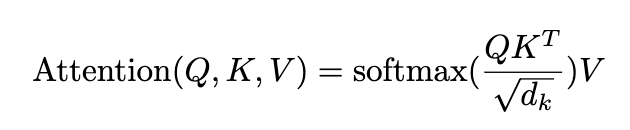
Attention can bee summarised with this formula you will find in the original paper. Now you might look at the original equation and ask what is the $\sqrt d_k$ part doing ? Essentially this just helps the attention values from growing too large, which can lead to vanishing gradients and instability.
Attention Computational Complexity
All of this computation is done via matrix multiplication, which is great because it allows to parallelise the calculations, but it also leads to one of the major limitation of transformers: the quadratic cost of attention. The amount of computation needed for the attention mechanism grows rapidly as the input size increases. This can make transformers very slow and expensive to run on long sequences of data.
Computational complexity two matrices of dimensions $m \times n$ and $n \times p$ is given by $O(m \cdot n \cdot p)$
In the context of the attention mechanism in neural networks, if we have a sequence of length $n$ and each vector is of dimension $d$, the multiplication of the query and key matrices (to compute the attention scores) has a complexity of $O(n^2 \cdot d)$. This is because we need to compute the dot product for each pair of query and key vectors, leading to $n^2$ operations for each dimension $d$.
Masked Self Attention
Masked self-attention is used in the decoder blocks of the Transformer model. Unlike the encoder’s self-attention, where each token can attend to all other tokens in the sequence, masked self-attention ensures that each position can only attend to earlier positions in the sequence (it sets future positions to -inf, effectively “masking” future tokens). This is crucial for autoregressive generation tasks, where the model generates tokens one at a time and must not peek at future tokens.
Cross-Attention (Encoder-Decoder Attention)
Cross-attention, is a key mechanism in the decoder blocks of the Transformer model that enables interaction between the encoder and decoder blocks. In this mechanism, the decoder generates queries ($Q$) from its own masked self-attention sub-layer output. These queries are then matched with keys ($K$) and values ($V$) produced by the encoder’s final output.

This connection allows the decoder to attend to the encoded representations of the input sequence, effectively integrating information from the source sequence into the target sequence generation process. By combining the encoded context from the encoder with the decoder’s own context, cross-attention ensures that the generated output is informed by the entire input sequence, enhancing the coherence and relevance of the translation or prediction.
Multi-Head Attention
Multi-head attention involves running multiple attention mechanisms in parallel. Each “head” operates on the same input data but with different learned weights, allowing the model to capture various aspects of the relationships between tokens. Think of it like multiple kernels in a convolutional neural network (CNN); each head can focus on different features or patterns in the data (i.e learning a different set of weights). The original paper uses 8 heads.
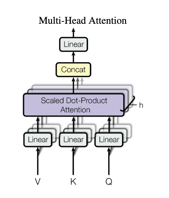
After processing the data in parallel through multiple heads, the outputs are concatenated together and then and linearly transformed back to the original dimensions. Here in the linear projection, we have the attention layers 4th learnable weight matrix, $W^O$. By concatenating the outputs first instead of summing them, and then projecting them back to the original dimensions, we can combine and mix the information in rich ways from different heads. This enhances the model’s ability to capture diverse and complex patterns in the data.
Fully Connected Layers, Layer Norm & Residual Connection
While these are the vanilla parts you’ll see in most architectures, it’s doing a quick review of what they are and the purpose they serve.
The feed-forward layers are fully connected neural networks that give the network it’s non-linear transformations / properties, allowing the model to extract much richer relationships.
Each sub-block (self-attention and feed-forward) is followed by layer normalisation and residual connections, which help stabilise training and improve performance.
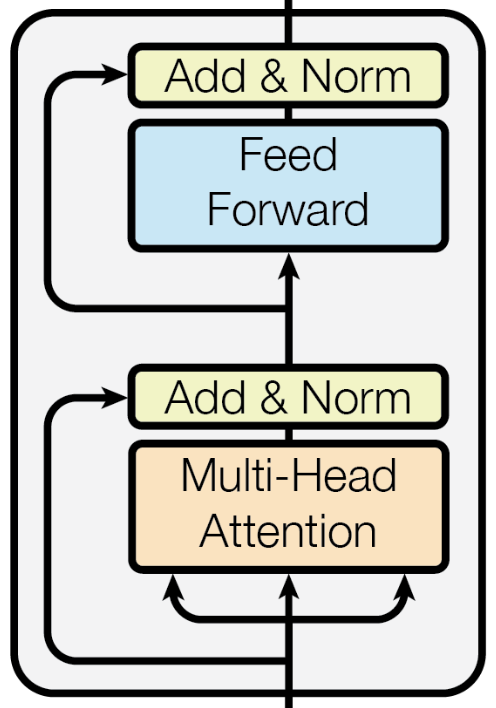
If you are not familiar with these concepts, layer normalisation ensures that the inputs to each sub-layer have a consistent distribution, which speeds up convergence and improves the model’s robustness. And residual connections add the input of a sub-layer to its output, allowing gradients to flow through the network more effectively during back-propagation, and avoid the vanishing gradient problem.
The combination of layer normalisation and residual connections helps maintain a stable training process and enhances the overall performance of the Transformer model.
Output Layer
So now that our input sentence has been translated into embeddings, and then gone through many blocks of encoding to learn dense representations and back out through the decoder layers, how do we get from decoder outputs to real generated text ?
The output of our last decoder block is a matrix of $M \times D$ (sequence length x embedding dimension). This output matrix undergoes a linear transformation. This is typically done using a fully connected layer, also known as the output projection layer. The purpose of this layer is to map the embedding dimension to the size of the output vocabulary.
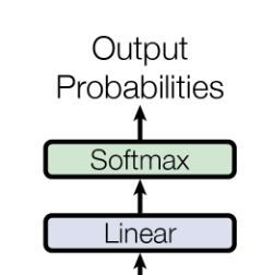
So we go from a $M \times D$ matrix to a $M \times V$ matrix. You can interpret this as each vector that represents an output token (of M token) has $V$ values, each entry being a score for the most likely word in our vocabulary.
We then pass this matrix through a softmax function to convert the raw scores (known as logits) to probabilities. In the training stage these probabilities are used to calculate the loss, and in the inference stage we can sample from the softmax distribution (from the vocabulary) using some sampling technique.
We can also tune the softmax function with a parameter called temperature that adjusts how confident or spread out the probability distribution is. This decides how creative or random our model is.
To understand better how the softmax function works you can check out this great YouTube video, Softmax Function Explained In Depth with 3D Visuals.
Wrap-up & Conclusion
Well, that’s it for the Transformer architecture. In this two-part series, we’ve covered the path from raw text to tokens to embeddings, explored the mechanics of attention, and circled back to raw text again. Along the way, we’ve touched on why the architecture is powerful due to parallelisation and issues like computational complexity. I hope this has shed some light on the inner workings of Transformers and how they’re revolutionising the way we process and understand language.