
- Introduction
- Inference Servers & Why We Need Them
- The phases of inference
- Key-Value Cache (KV Cache)
- GPU Bottlenecks for Inference
- End of Part 1
Introduction
Running LLMs in the real world is a complicated and expensive operation. Models are large in size and can be extremely compute and memory hungry. To run LLMs in a cost efficient way, and deliver outputs with speed (perhaps meeting some internal SLO) we need to know how to tune our model serving setup correctly. In this article we will go explore some of the tools developed for model inference, but mainly we will be deep diving into the optimisations these tools implement to ensure cost-effective and fast delivery of LLM outputs.
To understand this article properly, it’s expected you have a strong understanding of the Transformer architecture.
Inference Servers & Why We Need Them
Inference servers are specialised systems designed to efficiently run trained machine learning models. These servers are optimised for low latency and high throughput workloads. Basically to run our resource hungry LLMs effectively you this kind of specialised software to optimise at serving time, specifically tackling things like:
- Memory Optimisation
- Batching
- Parallelisation
- Transformer Specific Optimisations
- Specific GPU Support
- and many more…
A whole host of inference servers have appeared to cater to the requirements of serving LLMs:
- Triton Inference Server → An offering from NVIDIA which supports a number of DL frameworks and provides excellent support for GPU models & workloads
- vLLM → A standalone inference server, can be used as a backend in Triton, which provides a number of optimisations such as PagedAttention for Transformer models.
- LLama.cp → Specifically designed for deploying LLaMA models. Aimed to be easy to set up, purely in C/C++, so no dependencies, and comes with many optimisations for LLMs.
- Text Generation Inference → An offering from HuggingFace that integrates with their model repository. It provides support for both CPU and GPU deployments.
I plan to do a deep dive into the differences between the inference servers on offer in a subsequent blog post, but for now, just know that they are available and are here to make your life easier by implementing the optimisations we will talk about in this series of articles.
Let’s start by digging into how most LLMs work during inference.
The phases of inference
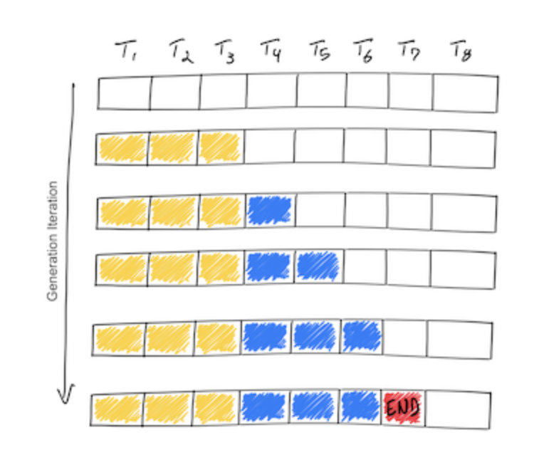
GPT based, or decoder only architectures, have 2 distinct phases when receiving a request from a client, a “pre-fill” phase and a “decode” phase. It’s crucial to understand how these phases work as we begin to examine the optimisations we can implement to speed up inference.
Pre-fill Phase
In the pre-fill phase, the model receives all the users input which makes it’s initial pass through the model. All the tokens are known up front and can therefore be processed in parallel, calculating the Query, Key, and Value matrices in the attention layer. The Key and Value matrices are cached for later use so they don’t need to be recalculated at each pass. We will look at this KV cache in more detail later. It’s also important to note that this phase also produces the first new token that is appended to the initial request.
Decode Phase
In the decode phase, we can no longer take advantage of parallelisation as each output value depends on the value before it. The decode phase repeats itself until it reaches an End token and token generation stops. This stage makes up most of the inference time, and due to it’s sequential nature, inference is much more memory bound than compute bound. Therefore, naturally the optimisations found in this article are geared towards this decoding phase.
The two stages can be summarised in the image below.
Measuring/Instrumenting Inference Stages
Not only is inference different in LLMs compared to traditional ML models due to it’s sequential nature, but it also comes with a host of it’s own metrics:
- Time To First Token (TTFT)
- Time Per Output Token (TPOT)
- Latency - The time to serve the full response
- Throughput - The number of tokens generated p/second
These are worth measuring and keeping track of when you deploy one of these models in production.
Key-Value Cache (KV Cache)
We mentioned the concept of the KV cache in the pre-fill phase of an LLM request. So, what is it and what problem does it solve?
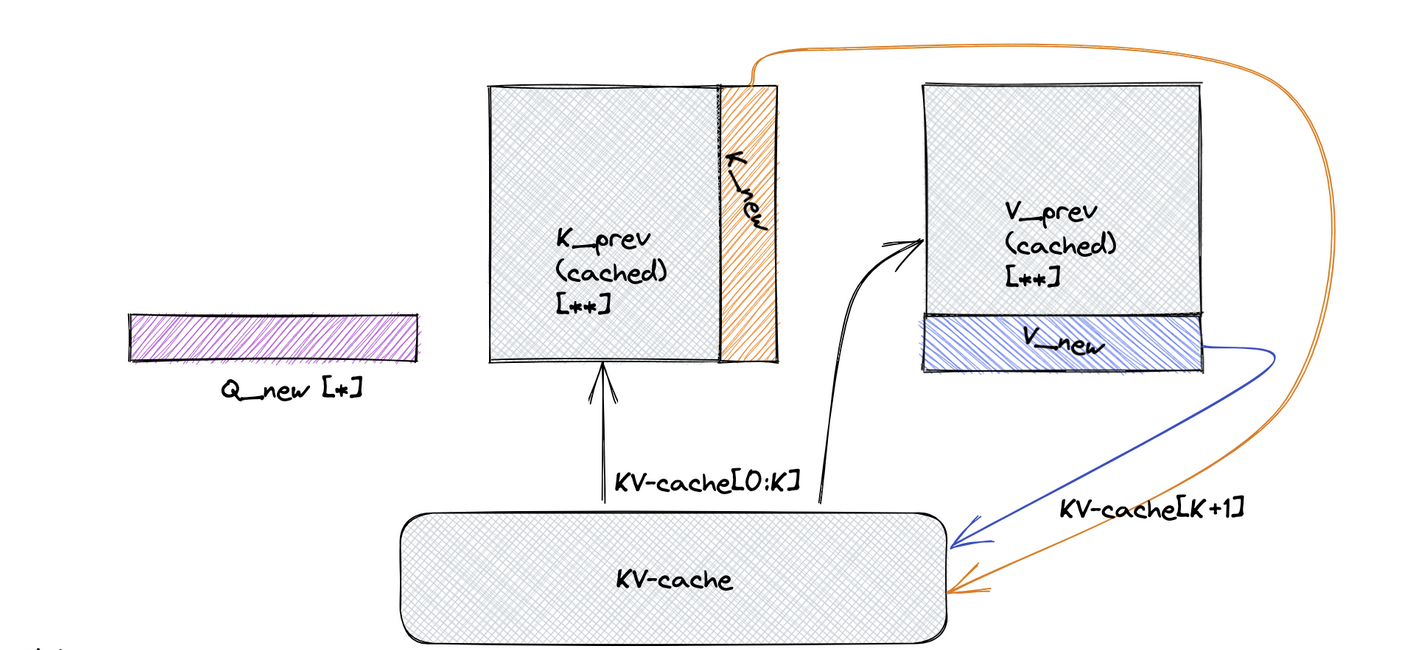
In essence, when we first take the user’s query/prompt, before we can begin generating new tokens, we need to calculate the $Q$, $K$, and $V$ values for each of the incoming tokens. However, to generate new tokens, we only need the $Q$ vector of the latest token and the $K$ and $V$ matrices of all previous tokens. Thankfully, we don’t need to calculate these values each time as they remain unchanged once calculated. When we calculate the initial matrices of $K$ and $V$, we store them in a cache for reuse later. Then, upon generating new tokens, we calculate the $K$ and $V$ vectors for the new token and append them to our already existing matrices for $K$ and $V$. This allows us to use the same resources at each decoding step.
GPU Bottlenecks for Inference
When it comes to LLM inference, most models are going to take advantage of GPUs ability to parallelise computation. Models can run on CPUs, but it won’t be the focus of this article.
One of the main ideas that we will run into again and again is that LLMs inference workload on GPUs is memory bound, compared to training which is limited by available FLOPs. Therefore we need to focus on using & managing memory as efficiently as possible to speed up & to reduce the cost of running LLMs in production.
Moreover, the trend for GPUs is that computation power is growing faster than memory. From the PagedAttention paper we will cover later:
…from NVIDIA A100 to H100, The FLOPS increases by more than 2x, but the GPU memory stays at 80GB maximum. Therefore, we believe the memory will become an increasingly significant bottleneck.
Calculating Memory Requirements
So how do we know how much memory our model will consume so we can provision the right hardware. There are two main things that occupy the majority of the memory requirements:
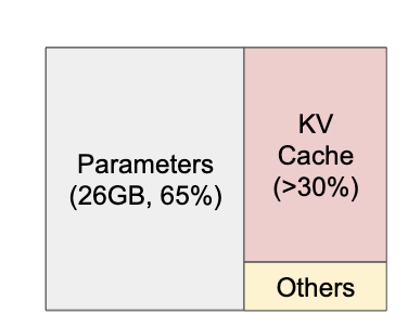
Model Weights → Typically consumes around 65% of the total memory requirements of serving. We can estimate the model size using the number of parameters and the floating point precision of each weight.
\[Model Size (bytes)=N Parameters×Parameter Size (bytes)\]- 32-bit floating point: Each parameter is 4 bytes.
- 16-bit floating point: Each parameter is 2 bytes.
- 8-bit integer: Each parameter is 1 byte.
As the Mistral model has 7 billion parameters, that would require about 14GB of GPU RAM in half precision (float16), since each parameter is stored in 2 bytes.
The KV Cache → Typically consume around 30% of the total memory requirements for serving. To get an idea of the absolute size a KV cache may need, we can calculate the space requirements per token:
\[2 (k \ and \ v \ vectors) × 5120 (hidden \ state \ size) × 20 (number\ of\ layers) × 2 (bytes \ per \ FP16) = 400kb\]Now if we had a mode that could generate sequences up to 8000 tokens, the memory required to store the KV cache of one request can be as much as 3.2 GB. GPUs only have memory capacities in the tens of GBs. So even if all available memory was allocated to KV cache, not a huge amount of requests could be accommodated.
End of Part 1
That concludes it for Part 1, we looked into the benefits inference servers can provide us, the phases for how LLMs process requests at inference, the bottlenecks seen in GPUs and how to calculate the memory footprint of our models for inference. Stay tuned for the rest of the series where we will cover attention mechanism optimisations, model compression strategies, distributed inference & batching strategies.
See part 2 of this series, A Guide to LLM Inference (Part 2): Attention Optimisation