
If you missed the start of this series please check it out from that start, A Guide to LLM Inference (Part 1): Foundations
Introduction
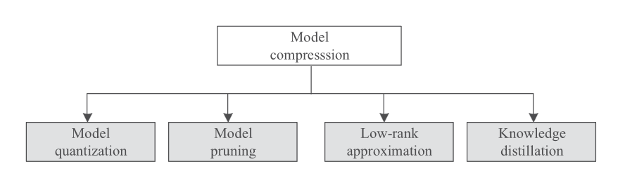
Model compression is a class of techniques that aim to reduce the size & complexity of models in order to make them easier and cost effective to deploy. We have a number of options available to reduce a models footprint, but they fall into the 4 general categories of either reducing precision, removing redundancy, transferring knowledge to smaller architectures or factorising representations. While each approach offers unique benefits, we’ll focus on the three most widely used techniques Model Quantization, Pruning and Distillation.
Quantization
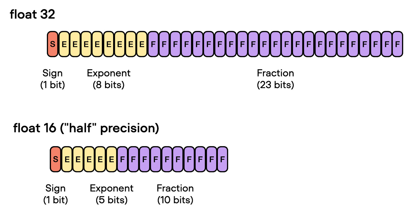
Model Quantization is one of the simplest techniques we can implement. The main idea being, that we reduce the precision of the models parameters. This in turn uses less memory and less CPU, making the model smaller and faster. For example, during model training we usually represent parameters of a model in FP32 precision (FP64 is overkill), and with compression, we can cut the model size almost in half by using FP16 precision, or even further to INT4 (4 bit integer). The more we reduce the precision the smaller and faster the model gets, but we make a tradeoff vs the quality of the outputs.
So what parts of the model do we quantize ? Normally it’s most common to quantize the weights, the activations and also the KV cache (HuggingFace has a nice article about KV cache quantization).
There are 2 main approaches to quantising models:
- Post-Training Quantization (PTQ) → This is the more naive and simple approach that involves converting the weights of a model that has already been trained. Because all we do is a simple conversion, performance degradation is a given, especially at lower precisions.
- Quantization-Aware Training (QAT) → During training time, we simulate how quantization will happen at inference time (by clipping / rounding values) and train a model that will loose minimal accuracy when quantised later. The tradeoff here is that it’s more computationally expensive to train.
Before finishing with quantisation, it’s interesting to note that research now is focused on seeing how extreme these techniques can be pushed, with a recent paper even training 1-bit LLMs with great results. There’s also a clear pattern emerging that larger parameter models seem to deal better with quantisation than smaller models, so once again, scale is our friend.
Pruning
Next in our arsenal of tools for model compression, we have pruning. Instead of reducing the footprint of parameters by representing them in lower precision, we just completely remove parts of the model. Of course as remove parts of the model, performance will naturally degrade. Therefore a host of strategies have been devised to best tackle this compression / performance tradeoff which will explore here.
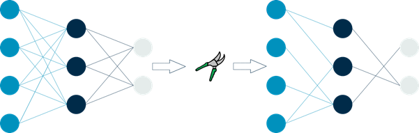
An example of weight pruning (Image Source)
In the review paper, What is the State of Neural Network Pruning?, they lay out the general algorithm for pruning and key characteristics that can help us differentiate between various pruning methods.
…the network is first trained to convergence. Afterwards, each parameter or structural element in the network is issued a score, and the network is pruned based on these scores. Pruning reduces the accuracy of the network, so it is trained further (known as fine-tuning) to recover. The process of pruning and fine-tuning is often iterated several times, gradually reducing the network’s size.

An example of an iterative pruning algorithm (Image Source)
Pruning Methods can be categorised based on several key characteristics:
- Scoring: This determines how we identify which parts of the model to prune. Common approaches include:
Random: Randomly selecting parameters to prune.Magnitude: Pruning based on the absolute value of weights, i.e, remove a certain percentage of parameters with the smallest magnitudes.Gradient-based: Using gradient information to determine importance. The core idea is that parameters with small gradients contribute less to the model’s output and are therefore good candidates for pruning. (Paper: Optimal Brain Surgeon)Regularization-based: Incorporating pruning into the loss function. We can use something as simple as L1 regularisation.
- Structure: Pruning can be either structured or unstructured:
Structured: Removes entire units (neurons, channels, or layers), maintaining the model’s regular structure but potentially limiting flexibility.Unstructured: Removes individual weights, offering more flexibility but potentially resulting in sparse matrices that are harder to optimise for hardware.
- Scheduling: This refers to when and how often pruning occurs:
One-shot: The model is pruned once after initial training.Iterative: Pruning is done in multiple rounds, often with fine-tuning in between.
It’s worth noting that these methods are not mutually exclusive and can often be combined for better results. After pruning, the model is typically fine-tuned to recover lost accuracy.
The approach to fine-tuning can vary:
From scratch: Resetting weights and retraining.Weight Rewinding: Rewinds unpruned weights to their values from earlier in training and retrains them from there using the original training schedule. (Paper: Comparing Rewinding and Fine-tuning)Continued training: Resuming training from the pruned state.
As with quantization, recent research has shown that larger models tend to be more robust to pruning, further emphasising the “bigger is better” trend in AI. However, the ultimate goal is to find the sweet spot between model size, computational efficiency and task performance.
So now we also have pruning as a powerful technique in the model compression toolkit. When used in conjunction with other methods like quantization and distillation, it can lead to significantly smaller and faster models without substantial loss in performance.
Distillation
The main idea is simple, we take a large language model (the teacher) that we want to use, and train a much smaller model (the student) to replicate it’s behaviour. It’s a simple but powerful idea. The original idea was introduced in a paper from Geoffrey Hinton called “Distilling the Knowledge in a Neural Network”. One of the best know examples is DistillBert (paper) which had impressive results. It reduced the original BERT model size by 40%, while maintaining 97% of the performance and speeding up inference by 60%!
So, how exactly does this work ?
In the case of a language model, we train the smaller model to minimise the loss on the output probabilities (obtained from applying a softmax function to the neural network outputs) between it and it’s teacher.
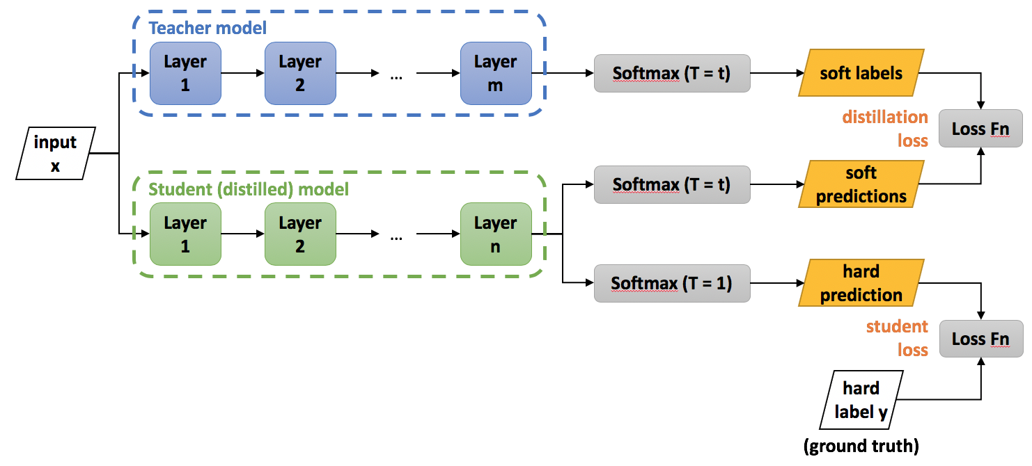
The process of model distillation (Image Source)
Let’s take a concrete example. Let’s say we are training on a sentence “Croissants are the king of pastries”, because they are! We get both models to predict a probability distribution over the vocabulary (soft labels), $P^T$ and $P^S$. For example, for simplicity let’s assume this sentence is our entire vocabulary, looking at the token “Croissant”, for each model we get the distribution
\[Teacher = P^T(Croissants)=[0.1,0.3,0.1,0.05,0.15,0.2,0.1]\] \[Student = P^S(Croissants)=[0.15,0.25,0.1,0.1,0.1,0.25,0.05]\]Now we can calculate some loss function over these distributions and try minimise this during the distillation process. Here we can use something like the Kullback-Leibler (KL) divergence. In addition to minimising the loss between the student & teach, we also try minimise the loss between the student and the ground truth labels, so our final loss function becomes (where $α$ is a weight factor that balances the two losses):
\[L=α⋅L_{distill}+(1−α)⋅L_{supervised}\]If you want to try this for yourself, IntelLabs has a python package for distilling larger models into smaller, lightweight and faster version, you can check it out, it’s called Neural Network Distiller.
End of Part 3
So we’ve explored three key model compression techniques:
- Quantization: Reducing parameter precision to decrease memory usage and computational needs.
- Pruning: Removing less important model parts through various strategies.
- Distillation: Training smaller models to mimic larger ones, transferring knowledge efficiently.
These methods, alone or combined, significantly reduce model size while aiming to preserve performance. Interestingly, larger models tend to be more resilient to compression, though the goal remains finding the optimal balance between size, efficiency, and performance.
If you missed the start of this series please check it out from that start, A Guide to LLM Inference (Part 1): Foundations